Retail Concepts
- Activity Ratios
- Assortment Planning
- Cumulative Markup Percentage
- Customer Segmentation
- Efficient Item Assortment (EIA) Model
- Financial Leverage Ratios
- Forecasting
- Geodemographics
- Gross Margin Percentage
- Individual Markup Percentage
- Inventory Management
- Markdowns Percentage
- Market Value Ratio
- Net Sales
Activity Ratios
Activity Ratios are used to measure how well a retailer's assets are being managed. To find out the right level of investment in assets, we can compare assets to yearly sales to calculate turnover, which shows how fast assets are used to generate sales. Total asset turnover is calculated by dividing total operating revenues by the average of total assets.
Total Asset Turnover = Total Operating Revenues ÷ Average Total Assets
If the asset turnover ratio is high, the retailer is using its assets well to generate sales. If the ratio is low, the retailer is not using their assets well and should either increase sales or get rid of some of the assets.
The receivables turnover ratio and the average collection period provide information on how well the retailer is managing its accounts receivables. The ratios suggest the retailer's credit policy. A liberal policy will result in a higher amount of receivables than with a restrictive policy. The average collection period should not be higher than the time allowed in the credit terms by more than 10 days.
The Ratios are calculated as:
Receivables Turnover = Total Operating Revenues ÷ Average Receivables
Average Collection Period = Days in Period ÷ Receivables Turnover
Inventory Ratios measure how fast inventory is produced and sold. Inventory turnover is calculated as the cost of goods sold divided by average inventory. The number of days in the year divided by the inventory turnover is the days in inventory ratio, which is the number of days to get merchandise produced and sold. It is also referred to as shelf life.
Inventory Turnover = Cost of Goods Sold ÷ Average Inventory
Days in Inventory = Days in Period ÷ Inventory Turnover
Example
The total operating revenues for a retailer are $2,134 million and it has average total assets of $1,709 million. Receivables are $279 million. Inventory is $280.75 million. The cost of goods sold is $1,533 million. What is the total asset turnover, receivables turnover, average collection period, average inventory, inventory turnover, and days in inventory.
Solution
Total asset turnover = Total Operating Revenues ÷ Average Total Assets
Total asset turnover = $2,134 ÷ $1,709
Total asset turnover = 1.25
Days in inventory = Days in Period ÷ Inventory Turnover
Days in inventory = 365 ÷ 5.46
Days in inventory = 66.8 days
Receivables for the year = $279
Receivables turnover = Total operating revenues ÷ Receivables
Receivables turnover = $2,134 ÷ $295
Receivables turnover = 7.60
Average collection period = Days in period ÷ Receivables turnover
Average collection period = 365 ÷ 7.60
Average collection period = 48.0 days
Average inventory = $280.75
Inventory turnover = Cost of goods sold ÷ Average Inventory
Inventory turnover = $1,533 ÷ $280.75
Inventory turnover = 5.46
Assortment Planning
Another component of category management is Assortment Planning. Customers want a good selection of the basic and specialty items available in the market to meet their needs. The goal of the retailer is to have just the right level of assortment: too many items and customers will perceive the assortment to be poor, and too many items and customers will be overwhelmed by the options.
The right mix satisfies customer needs while differentiating the retailer. This is one of major reasons that category management is conducted by retailers. It is to reduce out of stocks, maximize inventory efficiency, increase sales and increase margin of a brand.
The Category Assortment Plan defines the performance metrics for the category. The key metrics of the plan include:
- Average Revenue/Square Foot (sq ft)
- Gross Margin
- Average Ticket Size
- Stock to Cover Demand Forecast
- Product Alignment to Target Customer Profile
It is critical for the retailer to understand their customer's buying patterns. Defining the target customer's age, income, category preferences and other influences can significantly impact sales performance.
Within a category, shelf displays are typically planned by product and supplier/brand. Based on sales and market history, a sales projection is created which approves the inventory requirement needed to fill the shelves.
Cumulative Markup Percentage
It is more common to report markup percentage for a category, department, or class for a period of time.
Cumulative markup is the percentage difference between the total cost of a group of items and the total selling price of the group.
Cumulative markup is more useful when comparing the performance of items with defined goals, with past sales, or across categories, departments, classes or stores.
Cumulative Markup Percentage = Total Markup ÷ Total Retail
Buyers plan cumulative markup goals for items they manage. The cumulative markup percentage on a group of items is one of the most important goals for the buyer to plan. By defining their goal, the buyer can measure their performance. Often, buyers change their strategy when goals are not met.
By measuring their progress to their cumulative markup goal, buyers can make changes in their item pricing strategy before the end of the season when it would be too late.
Example
At the start of the summer season, a buyer's inventory of shorts had the following values:
Total Cost: $12,000
Total Retail: $17,600
During the month, the following purchases were made by the buyer:
60 shorts, costing $25 and selling at $45
90 shorts, costing $15 and selling at $30
Solution
| Cost | Retail | |
|---|---|---|
| Beginning inventory | $12,000 | $17,600 |
| Purchases | $1,500 (60 × $25) | $2,700 (60 × $45) |
| Purchases | $1,350 (90 × $15) | $2,700 (90 × $30) |
| Total | $14,850 | $23,000 |
Calculate total markup by subtracting total cost from total retail:
$23,000 − $14,850 = $8,150
Calculate cumulative markup percentage by dividing total markup by total retail:
$8,150 ÷ $23,000 = 35.4%
Customer Segmentation
Customer Segmentation is the process of dividing a market into unique customer groups that share characteristics. Customer segmentation is used to identify customer needs. Retailers that identify segments are better able to develop unique products and services and deliver product assortments that directly meet customer needs.
Customer Segmentation requires retailers to:
- Divide the market into measurable segments according to customer behaviors, demographic profiles, and needs.
- Determine the sales and margin potential of each segment by analyzing the impacts of selling to each segment.
- Target segments that they are able to serve in a competitive way.
- Invest in tailoring products, marketing, and distribution to match the needs of each segment targeted.
- Measure the performance of each segment and adjust the segmentations over time.
Example
For Besteck, seven distinct customer segments have been identified:
- Soccer Moms
Married, middle-class women that live in the suburbs and have school age children. - Wealthy Professionals
Upper middle-class to upper-class professionals, 35+ years old and with university degrees. High household income. - Tech Enthusiasts
Unmarried, middle-class men that live alone and are very tech savvy, often early adopters of new technology. - The Family Man
Married, middle-class men that live in the suburbs and have school age children. - The Small Business Customer
Middle aged, middle- to upper-class with high household income that owns their own business. - Young, Singles
Young, single and working professionals with no children that live downtown in apartments. - Older Couples Without Children
Older couples, often seniors, with children that no longer live at home. Lives in a house.
Efficient Item Assortment (EIA) Model
The Efficient Item Assortment Model (EIA) is a way to determine the optimal assortment of products in a category. The analysis comprises a six-step process that incorporates information from the retailer and supplier.
Six-Step Business Process
Step 1
Market Coverage: defines a target % for the sales contributed by products in a category. The target % is used to recommend: item retention, item deletion and item addition. Questions to determine the appropriate coverage level:
- How broad is the competitor's assortment?
- Does the consumer expect a broad or narrow assortment for the category?
- Can a higher coverage be achieved with a small assortment? Is product space being wasted on products that don't contribute much to the category?
- Is the category profitable enough for a higher coverage?
- Is the interest in a category growing or shrinking?
- Is there enough shelf space for a broad assortment of products? Does the assortment have to be reduced to fit the available space?
Step 2
Item deletion validation: justifies the deletion of products failing below the coverage target %.
Step 3
Item retention validation: determines whether or not to retain products that meet the coverage target %.
Step 4
Item addition validation: decides whether or not to add products that fall within the target % but are not in the current assortment.
Step 5
Assortment finalization: the validation steps to create a new assortment.
Step 6
Assortment qualification: estimates and compares the financial performance of the new and the current item assortment.
Financial Leverage Ratios
Financial Leverage measures how much a retailer is using debt financing instead of equity. Financial leverage ratios help to determine the likelihood that a retailer will default on its debt. The more debt a retailer has, the more likely it will not be able to meet its financial obligations. However, debt is a significant type of financing, and provides a tax advantage because interest payments are tax deductible.
Debt Ratios provide information about insolvency and the ability of the retailer to obtain more financing for investment opportunities. The debt ratio is calculated as total debt divided by total assets.
Debt ratio = Total debt ÷ Total assets
Debt equity ratio = Total debt ÷ Total equity
Equity multiplier = Total assets ÷ total equity
The Interest Coverage Ratio shows the ability of a retailer to generate sufficient income to cover interest expense.
The ratio is associated to the retailer's ability to pay interest. It is calculated as earnings (before interest and taxes) divided by interest expense.
Interest Coverage = Earnings before interest and taxes ÷ Interest expense
Example
A retailer has a total debt of $904 million with total assets of $1,643 million. Total equity is $702 million. Earnings before interest and taxes is $302 million and the interest expense is $38 million. What is the Debt ratio, debt equity ratio, and interest coverage?
Solution
Debt ratio = Total debt ÷ Total assets
Debt equity ratio = Total debt ÷ Total equity
Equity multiplier = Total assets ÷ total equity
Debt ratio = $904 ÷ $1,643
Debt equity ratio = $904 ÷ $702
Equity multiplier = $1,643 ÷ $702
Debt ratio = 0.55
Debt equity ratio = 1.29
Equity multiplier = 2.34
Interest coverage = Earnings before interest and taxes ÷ Interest expense
Interest coverage = $302 ÷ $38
Interest coverage = 7.95
Forecasting
Allocation and replenishment analysts have to use data to make forecasts about the future. Forecasting involves predicting what shoppers may do. Forecasts are typically made for consumer demand, sales and needed inventory levels.
Analysts typically create forecasts to answer questions such as:
- How Much product should be ordered?
- How Should product be allocated to stores?
- How Much inventory is needed for planned sales?
Sales Forecasts can include specific products, specific customers, time periods and specific store locations. A sales forecast should examine internal (advertising, prices, types of stores) and external (economic, demographic, competitive) forces. The micro and macroeconomic environment should be analyzed. Composition and lifestyle changes of the customer base are important to be followed. Current and new competitors and their promotional strategies should be regularly reviewed.
To generate sales forecasts, analysts need to find and use primary and secondary sources of information.
Primary data originates from the retailer and comprises of business records, specific research such as customer surveys and any form of internal data recorded by the retailer.
Secondary data is external information that may come from business publications, trade associations and third party data gatherers. A retailer must ensure that any secondary data used is recent, relevant and accurate.
The key steps to making a sales forecast are:
- Review past retail sales.
- Analyze the economic conditions.
- Analyze any changes in sales potential for products.
- Analyze any changes in strategies being used by the retailer or its competitors.
- Forecast the sales.
The analyst should regularly compare actual sales against the forecast to determine its accuracy and make adjustments as directed by management.
Example
Based on the information in the table below, forecast sales for April this year.
| Month | Sales Last Year | Sales This Year |
|---|---|---|
| January | $38,000 | $44,000 |
| February | $45,000 | $50,000 |
| March | $49,000 | $53,000 |
| April | $50,000 | ? |
Solution
First, calculate the percentage of sales increase or decrease for the first three months from the previous year: Percent increase/decrease in sales = Difference in sales from last year to this year ÷ Previous year
January = ($44,000 – $38,000) ÷ $38,000 = 15.8% increase
February = ($50,000 – $45,000) ÷ $45,000 = 11.1% increase
March = ($53,000 – $49,000) ÷ $49,000 = 8.2% increase
Sales are better than last year, however the percentage decreased from February to March. We should now review the direction of monthly sales in the current year.
January to February = ($50,000 – $44,000) ÷ $44,000 = 13.6% increase
February to March = ($53,000 – $50,000) ÷ $50,000 = 6.0% increase
Sales growth is slowing. Sales growth last year during the same period is:
March to April (Last Year) = ($50,000 – $49,000) ÷ $49,000 = 2.0% increase
The calculations suggest that the appropriate forecast for sales in April this year should be between 2.0% and 6.0%.
Geodemographics
Geodemographics is:
- One of the most commonly used data sources / type of segmentation for retail and marketing applications
- Based on the analysis of many variables to identify types of neighbourhoods (area typologies).
- Multi-dimensional classification of areas, not people
- Based on the simple assertion that:
- similar consumers with
- similar buying habits live in
- similar neighbourhoods
- The analysis of people by where they live that acts as a powerful discriminator of consumer behavior.
- Consumer households close together are more likely to be similar than those far away (based on Tobler's 1st Law of Geography).
- Allow inferences to be made about behavior – if you know where someone lives you can make assumptions about the type of consumer they are.
What can you do with Geodemographics?
Identify the following:
- WHO your customers are
Profile of existing customers to identify the dominant segments - WHERE to find more of them
Identify areas that have an appropriate mix of the 'right' type of consumer (i.e., areas that match your customer profile) - HOW to reach them effectively
Target where to distribute flyers or open new stores / change store format
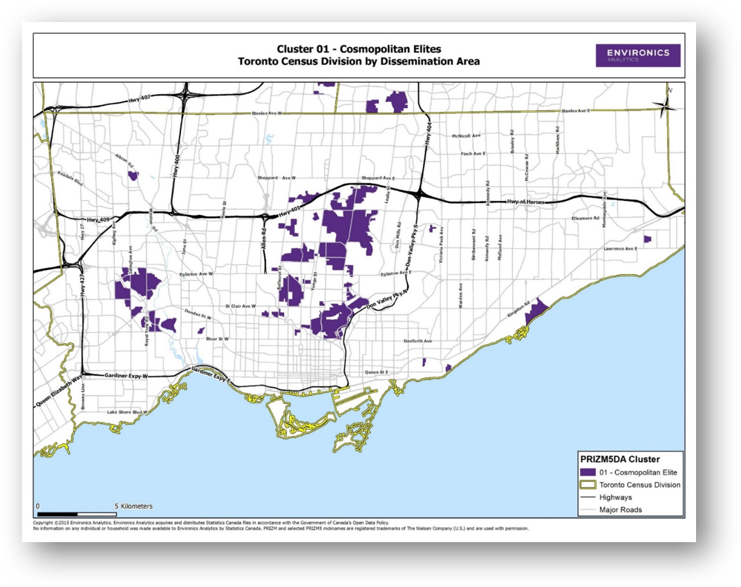
Figure 1: An example of a Geodemographic Cluster in Toronto (Source: Toronto Metropolitan University)
Gross Margin Percentage
Gross Margin is the sales revenue that remains after the cost of goods sold has been deducted.
Gross Margin = Total Net Sales – Cost of Sales
Gross Margin is a retailer's total net sales revenue minus its cost of sales. The gross margin represents the total sales revenue that the retailer retains after incurring the direct costs associated with producing the goods and services sold. The higher the number, the more the company retains on each dollar of sales to service its other costs and obligations. The gross margin percentage is the gross margin divided by total net sales, expressed as a percentage.
Example
The total net sales of the Drinkware department is $13,678. The cost of sales for the drinkware department is $6,927. What is the gross margin percentage of the Drinkware department?
Solution
Gross Margin % = (Total Net Sales – Cost of Sales) ÷ Total Net Sales
Gross Margin % = ($13,678 – $6,927) ÷ $13,678
Gross Margin % = 0.49357
Gross Margin % = 49.4%
Individual Markup Percentage
Markup is the difference between the cost of an item and its selling price. The markup is added onto the cost in order to create a profit for the retailer. The actual selling price may be lower than retail price due to sales. So the actual markup is on the price paid by the customer at purchase.
Markup % = (Retail – Cost) ÷ Retail
While the dollar amount of markup is important, the markup percentage is usually more important. Retailers typically state performance standards in percentage instead of dollars. Percentages are also better to compare the performance of multiple departments that may have very different price ranges.
Example
An item cost a retailer $35.86. If the item sells for $93.99, what is the markup percentage?
Solution
Markup % = (Retail – Cost) ÷ Retail
Markup % = ($93.99 − $35.86) ÷ $93.99
Markup % = ($58.13 − $35.86) ÷ $93.99
Markup % = $58.13 ÷ $93.99
Markup % = 61.8%
Inventory Management
One of the most important parts of category management is inventory management. It means maintaining the right amount of inventory at the right time. Too little inventory results in stock outs and not meeting customer demand. Too much inventory leads to markdowns and financial loss.
There are two common inventory management systems, known as "push" and "pull".
PUSH
Inventory in a PUSH system is managed corporately, where all buying decisions are made and then pushed to the distribution centre for allocation to stores.
The biggest benefit of a push system is the reduction of shipping costs. Push systems mean placing larger, less-frequent orders which reduces the number of shipments. However, inaccurate projections can leave a retailer over- or under-supplied. Over supply leads to markdowns, under supply leads to lost sale. Larger store space is required to store the larger orders.
PULL
Inventory in a PULL system involves store requirements to be consolidated at the corporate level through the distribution centre and then obtained by the stores.
A push system relies on placing smaller, more frequent orders. A pull system is more reactive to customer buying trends given that shelf stock is monitored in real-time and then ordered as needed by the store.
The main advantage of a pull system is that a retailer is better able to meet consumer demand without excess inventory. Changes in product demand can be met quickly. However, shipping costs can be high and sudden dramatic increases in a product's popularity can leave the retailer out of stock.
Choosing the right inventory management system for a retailer depends on several factors, including the type of retailer, quantity of inventory, warehouse and store space, and consumer demand. Regardless of the system, the primary goal is for the retailer to keep the shelves stocked with merchandise, minimize shipping costs, and increase margins.
Markdowns Percentage
Buyers need to know about the number and dollar amount of markdowns that have been taken. A markdown is the reduction in the retail price of an item that is in stock at a retailer. Knowing about markdowns tells the buyer which items have to be marked down to generate sales or should be purchased in lower quantities.
Buyers are interested in the markdown percentage during a season, which is the percentage reduction in the retail price of items that are in stock.
Items are often marked down because:
- Prices are reduced because the buyer purchased too much inventory based on the demand for an item.
- Items are priced higher than customers are willing to pay.
- Items are poorly merchandised within a store.
- To clear out remaining inventory at the end of the season.
Example
80 t-shirts were purchased for $20 each and sold at $40. At the end of the summer season, 20 t-shirts were left, which were marked down to $25 and sold. Total markdowns are $300 (20 t-shirts with a $15 markdown). Total sales were $2,900 ($2,400 for 60 t-shirts at $40 each plus $500 for 20 t-shirts at $25 each). The markdown percentage is calculated as follows:
Solution
Markdown % = Dollar markdown ÷ Total sales
Markdown % = $300 ÷ $2,900
Markdown % = 0.10345
Markdown % = 10.3%
Market Value Ratio
The Market Price of a share of common stock is the price that the stock trades at. The market value of the retailer is the market price of a share multiplied by the number of outstanding shares.
The Price-Earnings (P/E) Ratio is the ratio of the stock's market price to its annual current earning per share. The P/E ratio demonstrates how much investors are willing to pay for $1 or earnings per share.
Similar to P/E, Dividend Yield is related to the perception the market has for a retailer's future growth prospects. A retailer with high growth prospects tends to have lower dividend yields. It is calculated by annualizing the last dividend payment of a retailer and dividing by the current market price.
Dividend Yield = Dividend per share ÷ Market price per share
Example
A retailer has a market price per share of $35.86 and an annualized dividend per share of $1.23. What is the dividend yield?
Solution
Dividend yield = Dividend per share ÷ Market price per share
Dividend yield = $1.23 ÷ $35.86
Dividend yield = 0.0343 (3.43%)
Net Sales
Net Sales are the amount of sales generated by a retailer after the deduction of returns and allowances for damaged or missing goods, any discounts allowed and returns made by customers.
Net Sales = Gross Sales – Returns and Allowances – Customer Returns
The sales number reported on a retailer's financial statements is a net sales number, reflecting these deductions.
Example
The gross sales of the Office Supplies department is $43,250. There are $5,000 of damaged goods and customers returned $6,750 worth of items. What is the net sales of the Office Supplies department?
Solution
Net Sales = Gross Sales – Returns and Allowances – Customer Returns
Net Sales = $43,250 − $5,000 − $6,750
Net Sales = $31,500
New Store Location Selection
If you have not worked through Module 4: Developing a New Store Plan already, please refer to the business situation in that module for further context on this topic.
The Store Ranking Target Groups generates the rankings of the three key metrics needed to determine and compare the magnitude of potential demand for each store location. But which of the three (%, the % Pen, and Index) should be used to select the 6 new stores?
While any one of the three metrics can appear to be good on its own, it may not appear as great when applied within the context of other two metrics. For example, a store may have a high number of households (count), which is desirable, but have a low percentage (penetration) of households with the store's trade area. Or consider a store with a lower number of households (count). This is not highly desirable on its own, however the location may have a high index so most of the households in that location are the customers in the target group.
The best way to determine the appropriateness of a location is to review multiple metrics together, and select the location that provides the best overall combination of the three key metrics.
The store selection analysis brings together only the %, the % Pen, and Index metrics for the 18 potential store locations for the Suburban and Urban Core segments so that they can be compared to determine the best overall store locations for each core segment.
Optimization Problem
An optimization problem is one where you need to make the best decision based on a set of constraints. Solvers, or optimizers, are a type of software that helps determine what is the best outcome for a problem.
The problem might be allocating inventory dollars to stores, locating a new warehouse, or determining the optimal pack size. In each case, there could be many different viable solutions. However, you want to find the optimal solution while simultaneously satisfying a number of logical conditions (constraints). The optimal solution may be maximizing a variable (profits), minimizing a variable (costs), or achieving a particular outcome.
How to Use a Solver
In order to use a solver, you must build a model of your decision problem that specifies:
- The decisions to be made – decision variables
- The measure to optimize – the objective
- Any logical restrictions on solutions – constraints
The solver will find values for the decision variables that satisfy the constraints while optimizing (maximizing or minimizing) the objective.
Using Microsoft Excel is a convenient way to build an optimization model. The worksheet can contain numbers, labels, or formulas. The decision variables can be cells containing numbers the solver can change. The objective is a cell containing a formula you want the solver to maximize (or minimize) by adjusting the values of the decision variable cells. Constraints are logical conditions on formula cells that must be satisfied.
Steps Involved in Solving Optimization Problems
- Understand the problem that needs to be solved.
- Formulate the problem in words, including decision variables, objective function, and constraints.
- Develop the algebraic formulation of the problem.
- Define the decision variables
- Write the objective function
- Write the constraints
- Create a spreadsheet model.
- Set up the solver and solve the problem.
- Examine the results and update and refine the model.
- Analyze and interpret the results.
Pack Optimization
When retailers order and ship products, they are packaged together in what is referred to as packs, or a collection of items. A pack is typically a quantity of a single SKU, or a multiple units of similar SKUs (such as different sizes of the same style and colour shoe). Retailers group multiple units of one or more stock keeping units (SKUs) to reduce distribution and handling costs. However, ordering flexibility at the retail outlet is limited given that multiple items are grouped together.
The objective of Pack Optimization is to build the best possible combination of packs to meet each store's demand based upon the available packs. It means sending the right units to the store. Retailers that better manage size generate better margins than comparable retailers.
Pack Optimization is the process to find the best combinations of packing configurations to fill size demand in stores. The process uses size profiles and a number of variables and constraints, such as price, promotions, seasonality, inventory and shipping requirements.
Step 1
The first step is to create a size profile, typically by store, for a specific merchandise category. The size profiles are compared with assortment plans to generate purchase orders. The merchandise then arrives at a distribution centre in prepackaged cartons (boxes). Each carton typically contains a standard ratio of sizes. For example, a pack of 100 women's shoes may contain 10 size 6.5, 20 size 7, 50 size 7.5, and 20 size 8, packaged in sets of 10.
Given these pack configurations, and knowing how much of each size is required by store, what is the most efficient way to distribute the packs? In a large retailer with many stores and many different items, this can be very complex calculation that tries to align packs with customer demands, logistical costs and organizational constraints.
Different forms of dedicated software exists to automate the pack size process. The process begins by comparing the current size profile for each store against available inventory in the warehouse. This is important, as warehouse inventory is constantly changing, or a vendor may have shipped an incorrect quantity of merchandise.
Step 2
Then, an analysis evaluates all of the variables and constraints that the retailer has placed into the process and returns an optimized allocation for sending packs to stores. Advanced Analysis will need to answer questions such as:
- Should a whole pack be sent to stores?
- How many packs and to which stores?
- Does it make financial sense to break open a pack and send a smaller amount or even individual units?
The analysis should determine the precise number of packs needed to economically meet demand so that the retailer can maintain reasonable distribution costs, maximize sales and minimize out of stocks.
Planned BOM Inventory
The stock-to-sales ratio shows how planned sales are related to the inventory needed for those sales and is used to calculate planned beginning of the month (BOM) stock levels. This is the amount of stock needed to begin the month.
You can determine the amount of inventory needed at the beginning of the month by multiplying the stock-to-sales ratio for the month by the planned sales for the month.
Stock-to-sales ratio for the retail industry are available from multiple sources such National Retail Federation (NRF). Analysts can calculate the stock-to-sales ratio for their company based on previous stock to sales levels.
Example
Calculate the planned BOM inventory for September using the following information:
Stock-to-sales ratio = 2.6
Planned sales for September = $29,000
Solution
Planned BOM inventory = Stock to sales × Planned sales
Planned BOM inventory = 2.6 × $29,000
Planned BOM inventory = $75,400
Therefore, the retailer would want to start the month of September with $75,400 of inventory.
Planned EOM Inventory
The EOM (End-of-Month) stock for a month is the planned BOM (Beginning-of-Month) stock for the following month.
Example
For the six-month buying plan, planed EOM inventory would look like:
February EOM = $28,890 (March BOM)
March EOM = $42,693 (April BOM)
April EOM = $34,561 (May BOM)
May EOM = $22,363 (June BOM)
June EOM = $21,186 (July BOM)
July EOM = ...
We don't know the planned EOM for July because the BOM stock for August is unknown. The planned EOM for July is estimated at $20,000.
The calculated EOM inventory would then be entered in the six month buying plan on the Planned line.
| EOM | February | March | April | May | June | July | Totals |
|---|---|---|---|---|---|---|---|
| Last Year | $29,400 | $41,300 | $28,700 | $16,500 | $15,200 | $14,900 | $146,000 |
| Planned | $28,890 | $42,693 | $34,561 | $22,363 | $21,186 | $20,000 | $169,693 |
| Revised | |||||||
| Actual |
Planned Purchases at Cost
The initial markup for the period is 42.7 percent. Planned purchases at cost is calculated as follows:
Planned purchases at cost = (100% − Initial Markup %) × Planned purchases at retail
Planned Purchases at Cost can be calculated as follows:
| Month | (100% − Initial Markup %) | Planned Purchases at Retail | Planned Purchases at Cost |
|---|---|---|---|
| February | (100% − 42.7%) | × $12,524 | = $7,176 |
| March | (100% − 42.7%) | × $24,928 | = $14,284 |
| April | (100% − 42.7%) | × $13,208 | = $7,568 |
| May | (100% − 42.7%) | × $7,258 | = $4,159 |
| June | (100% − 42.7%) | × $12,123 | = $6,946 |
| July | (100% − 42.7%) | × $12,392 | = $7,101 |
The calculated planned purchases at cost would then be entered in the six month buying plan on the Planned Line.
Planned purchases at cost are used by the buyer to determine how much money they can spend on inventory for the season by month.
| Planned Purchases at Cost | Feb | March | April | May | June | July | Totals |
|---|---|---|---|---|---|---|---|
| Last Year | $6,674 | $13,213 | $7,061 | $3,897 | $6,453 | $6,576 | $43,873 |
| Planned | $7,176 | $14,284 | $7,568 | $4,159 | $6,946 | $7,101 | $47,234 |
| Revised | empty cell |
empty cell |
empty cell |
empty cell |
empty cell |
empty cell |
empty cell |
| Actual |
Planned Purchases at Retail
| Planned Sales | Planned EOM | Planned Reductions | Planned BOM at Retail | Planned Purchases at Retail | |
|---|---|---|---|---|---|
| February | $8,560 | + $28,890 | + $754 | − $25,680 | = $12,524 |
| March | $10,700 | + $42,693 | + $425 | − $28,890 | = $24,928 |
| April | $20,330 | + $34,561 | + $1,010 | − $42,693 | = $13,208 |
| May | $18,190 | + $22,363 | + $1,266 | − $34,561 | = $7,258 |
| June | $11,770 | + $21,186 | + $1,530 | − $22,363 | = $12,123 |
| July | $11,770 | + $20,000 | + $1,808 | − $21,186 | = $12,392 |
The planned purchases per month should be sufficient to execute the six month buying plan. Purchases are planned at retail first because all of the other metrics are based on retail.
Planned Purchases are calculated as:
Planned Purchases = Planned Sales + Planned EOM + Planned reductions − Planned BOM
Example
The calculated Planned Purchases would then be entered in the six month buying plan on the Planned line.
| Planned Purchases at Retail | February | March | April | May | June | July | Totals |
|---|---|---|---|---|---|---|---|
| Last Year | $11,560 | $23,009 | $12,191 | $6,699 | $11,190 | $11,438 | $76,087 |
| Planned | $12,254 | $24,928 | $13,208 | $7,258 | $12,123 | $12,392 | $82,433 |
| Revised | |||||||
| Actual |
Planned Reductions
The next step in the six month buying plan is planned reductions. Reductions include markdowns, employee discounts and shrinkage. Estimates based on history are provided as a percent of planned sales.
Example
Planned markdown percentage = 6.5%
Planned employee discount percentage = 1.4%
Planned shrinkage percentage = 1.1%
The total reductions are planned to be 9 percent of sales.
The total reductions is calculated by multiplying total planned sales by the reduction percent.
Total reductions = $81,320 x 9% = $7,319
Based on retailer history, the buyer has calculated reductions per month as the following:
| February | 10.3% |
|---|---|
| March | 5.8% |
| April | 13.8% |
| May | 17.3% |
| June | 20.9% |
| July | 24.7% |
The planned reductions are calculated as follows:
| % Reductions Planned for the Month | Total Planned Reduction | Planned Monthly Reductions | |
|---|---|---|---|
| February | 10.3% | × $7,319 | = $754 |
| March | 5.8% | × $7,319 | = $425 |
| April | 13.8% | × $7,319 | = $1,010 |
| May | 17.3% | × $7,319 | = $1,266 |
| June | 20.9% | × $7,319 | = $1,530 |
| July | 24.7% | × $7,319 | = $1,808 |
The calculated reductions would then be entered in the six-month buying plan on the Planned line.
| Reductions | February | March | April | May | June | July | Totals |
|---|---|---|---|---|---|---|---|
| Last Year | $712 | $406 | $956 | $1,134 | $1,375 | $1,623 | $6,206 |
| Planned | $754 | $425 | $1,010 | $1,266 | $1,530 | $1,808 | $6,792 |
| Revised | |||||||
| Actual |
Planned Sales
The first part of a six month buying plan is forecasting sales. All decisions are planned in relation to sales. If the sales forecast is wrong, all other components of the plan will be wrong.
Step 1
Obtain sales from the previous year's buying plan:
| Sales | February | March | April | May | June | July | Totals |
|---|---|---|---|---|---|---|---|
| Last Year | $8,000 | $10,000 | $19,000 | $17,000 | $11,000 | $11,000 | $76,000 |
| Planned | |||||||
| Revised | |||||||
| Actual |
Step 2
Calculate last year's monthly sales as a percentage of last year's total sales.
| Sales Last Year | Total Sales Last Year | % of Sales Last Year | |
|---|---|---|---|
| February | = $8,000 | ÷ $76,000 | = 10.5% |
| March | = $10,000 | ÷ $76,000 | = 13.2% |
| April | = $19,000 | ÷ $76,000 | = 25.0% |
| May | = $17,000 | ÷ $76,000 | = 22.4% |
| June | = $11,000 | ÷ $76,000 | = 14.5% |
| July | = $11,000 | ÷ $76,000 | = 14.5% |
Assuming no significant changes in the current season and a constant percentage of total sales, the buyer will plan for these percent of sales to occur each month.
Step 3
Determine the total planned sales volume for the season. Assuming a 7% sales increase from the previous year:
Planned Total = Last Year x (1 + Increase)
Planned Total = $76,000 x (1 + 7%)
Planned Total = $81,320
| Planned % of Total | Planned Total | Planned Monthly Sales | |
|---|---|---|---|
| February | 10.5% | × $81,320 | = $8,560 |
| March | 13.2% | × $81,320 | = $10,700 |
| April | 25.0% | × $81,320 | = $20,330 |
| May | 22.4% | × $81,320 | = $18,190 |
| June | 14.5% | × $81,320 | = $11,770 |
| July | 14.5% | × $81,320 | = $11,770 |
Solution
The calculated Planned Monthly Sales would then be entered in the six-month buying plan on the Planned line.
| Sales | February | March | April | May | June | July | Totals |
|---|---|---|---|---|---|---|---|
| Last Year | $8,000 | $10,000 | $19,000 | $17,000 | $11,000 | $11,000 | $76,000 |
| Planned | $8,560 | $10,700 | $20,330 | $18,190 | $11,770 | $11,770 | $81,320 |
| Revised | |||||||
| Actual |
Planogram Facings
Creating planograms are a time intensive process. An accurate, manually created planogram often takes over three hours to complete. Therefore, retailers often use commercial software such as JDA, to provide the ability to create views of the shelves, handle different products, and provide analysis reporting. However, even with software, planograms still require significant human input.
Shelf Space Allocation is the term used to describe how to distribute finite shelf space in a store to a group of products in a category. This depends on the type of retailer, company strategy, store layout, store size, another characteristics of the retailer.
A retailer usually displays only a limited amount of inventory of a SKU on the shelf. Where availability exists, excess inventory sits in the backroom. The stock visible on the shelves can be described by the number of facings wide, high and deep, as shown in the following illustration. The number of facings wide is typically referred to as the facings of the item. Orientation describes the way each product is placed on the shelves – front, back, top or side.
Store Fixtures are in groups and horizontally stacked against each other to create the aisles in the store. Each group has its own shelf arrangement. The shelves in one group can be aligned with the shelves in other groups to create long shelves from one end of the aisle to another.
Planogram Facings may also use fixtures other than shelves, including bins, baskets and pegboards. Bins are used to display non-organized products that do not stack well and pegboards are bars with steel rods that are used to hold peggable products like packages of batteries.
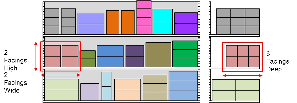
Figure 2: Planogram Facings (Source: Toronto Metropolitan University)
Price Elasticity
Most customers are sensitive to the price of a product. Typically, more people will buy a product if it is cheap and less will buy it if it is expensive. Price Elasticity shows how responsive customer demand is for a product based on its price. Retailers need to understand how elastic or inelastic their products are when making pricing decisions. Price elasticity is calculated as:
Elasticity = % change in quantity demanded ÷ % change in price
There are five zones of elasticity:
- Perfectly elastic – a very small change in price results in a very large change in the quantity demanded.
- Relatively elastic – small changes in price cause large changes in quantity demanded. Elasticity is greater than 1.
- Unit elastic – any change in price is matched by an equal change in quantity. Elasticity is equal to 1.
- Relatively inelastic – large changes in price cause small changes in demand. Elasticity is less than 1.
- Perfectly inelastic – the quantity demanded does not change when the price changes.
If elasticity is positive, then an increase/decrease in price will result in an increase/decrease in sales. If elasticity is negative, an increase/decrease in price will result in a decrease/increase in price. For products with price elasticity less than -1, the price that maximizes profits (optimized price) is calculated as:
Profit maximizing price = (Price elasticity x cost) ÷ (price elasticity + 1)
Example
A retailer originally priced a blender at $80 and then raised the price to $90. Before raising the price, the retailer was selling 750 units a week. When the price was increased, sales dropped to 600 units per week. What is the price elasticity of the blender?
Solution
Elasticity = % change in quantity demanded ÷ % change in price
Elasticity = ((New quantity sold – old quantity old) ÷ (old quantity)) ÷ ((new price – old price) ÷ (old price))
Elasticity = ((600 – 750) ÷ 750) ÷ ((90 – 80) ÷ 80)
Elasticity = -0.2 ÷ 0.125
Elasticity = -1.6
Price elasticity is a negative number because when the priced was raised the number of units sold decreased.
Profit Percentage
The profit is the amount of money that a retailer makes after operating expenses are subtracted from gross margin. If the operating expenses of a retailer are higher than the gross margin, there is a loss. If the gross margin is higher than the operating expenses, there is a profit.
The profit percentage expresses a retailer's profit as a percentage of the total sales revenue generated. As a percentage, it allows buyers to compare the profits of different departments that can vary greatly in size.
Example
The total sales of the Home Office department are $28,000. The Gross Margin is $20,000. The operating expenses of the Home Office department are $13,000. What is the profit percentage of the Home Office department?
Solution
Profit % = Profit ÷ Total Sales
Profit % = (Gross Margin – Operating Expenses) ÷ Total Sales
Profit % = ($20,000 – $13,000) ÷ $28,000
Profit % = $7,000 ÷ $28,000
Profit % = 0.2500
Profit % = 25%
Profitability Ratios
Accounting Profit is essentially the difference between revenue and costs. There is no completely clear way to know if a retailer is profitable. A financial analyst can measure accounting profitability, but depending on the strategy or time of the year, current profit may not accurately reflect future profitability.
Net Profit Margin reflects a retailer's ability to sell inventory at a higher price than its cost. It is calculated as net income divided by total operating revenue.
Net Profit Margin = Net income ÷ Total operating revenue
A common measure of managerial performance is the Return on Assets. It is the ratio of income to average total assets, both before tax and after tax.
Net return on assets (ROA) = Net income ÷ Average total assets
Gross return on assets (ROA) = Earnings before interest and taxes ÷ Average total assets
Retailers can increase ROA be increasing profit margins or asset turnover. Most retailers will trade-off between turnover and margin.
Return on Equity (ROE) is calculated as net income after interest and taxes divided by the average common shareholder's equity.
Return on Equity (ROE) = Net income ÷ Average shareholders' equity
The payout ratio is the proportion of net income paid out as cash dividends. It is calculated as cash dividends divided by net income.
Payout ratio = Cash dividends ÷ Net income
Example
A retailer has a net income of $197 million with total operating revenue of $2,134 million. Total assets are $1,709 million. Earnings before interest and taxes is $302 million. Shareholders' equity is $784.5 million. Cash dividends is $67 million. What is the net profit margin, net return on assets (ROA), gross return on assets (ROA), return on Equity (ROE), and payout ratio.
Solution
Net profit margin = Net income ÷ Total operating revenue
Payout ratio = Cash dividends ÷ Net income
Net profit margin = $197 ÷ $2,134
Payout ratio = $67 ÷ $197
Net profit margin = 0.092 (9.2%)
Payout ratio = 0.34
Net return on assets (ROA) = Net income ÷ Total assets
Net return on assets (ROA) = $197 ÷ $1,709
Net return on assets (ROA) = 0.115 (11.5%)
Gross return on assets (ROA) = Earnings before interest and taxes ÷ Total asset
Gross return on assets (ROA) = $302 ÷ $1,709
Gross return on assets (ROA) = 0.177 (17.7%)
Shareholders' equity = $784.5
Return on Equity (ROE) = Net income ÷ Shareholders' equity
Return on Equity (ROE) = $197 ÷ $784.5
Return on Equity (ROE) = 0.251 (25.1%)
Reverse Auctions
What Does This Mean?
In regular auctions multiple buyers attempt to out-bid each other for a certain product that eventually goes to the one with the highest bid.
In Reverse Auctions, sellers compete with each other to offer the lowest price they can in order to get a single buyer's business.
Example
A buyer at a major retailer needs to find a supplier who can offer snow shovels for the upcoming winter season. The buyer knows of 10 different suppliers who offer products in this category so he/she sets up a reverse auction indicating the specifications required for the shovel and invites all the suppliers to submit their lowest price possible to win the business. The buyer might not choose the absolute lowest price if other factors are considered - such as how long the shipment times are, or if there are other incentives offered by the supplier - but price is one of the key factors in a reverse auction.
The Auction Dashboard
An Excel-based dashboard can help to visualize and rank vendor bids by various selection criteria or considerations.
This dashboard contains a collection of charts for quick analysis including a bar graph showing the current bid in dollars per unit, a pie chart showing a breakdown of annual sales by vendor, and additional visual information as customized by the user.
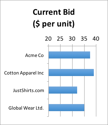
Figure 3: Current Bid (Source: Toronto Metropolitan University)
Figure 3 is a graph that shows the current bid in dollars per unit of four companies. It shows that Acme Co has a current bid of 37.5 dollars per unit, Cotton Apparel Inc. has a current bit of 38 dollars per unit, Justshirts.com has a current of 32 dollars per unit and Global Wear Ltd. has a current bid of 35 dollars per unit.
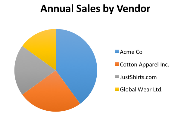
Figure 4: Annual Sales by Vendor (Source: Toronto Metropolitan University)
Figure 4 shows a pie of each company's annual sales. Acme Co has a share of 37%, Cotton Apparel Inc. has a share of 25%, Justshirts.com has a share of 22%, and Global Wear Ltd. has a 16%.
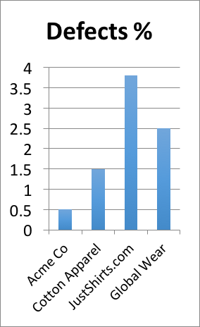
Figure 5: Defects percentage (Source: Toronto Metropolitan University)
Figure 5 is a diagram that shows the percentage of defects. Acme Co has a defects percentage of 0.5, Cotton Apparel Inc. has a defects percentage of 1.5, Justshirts.com has a defects percentage of 3.75 and Global Wear Ltd. has a defects percentage of 2.5.
Segmentation
What is Segmentation?
- Consumer behaviour is complex and diverse.
- Different consumers respond differently to the same stimulus.
- Different groups of consumers respond differently to the same stimulus.
- These groups can be identified with respect to any given product or service through segmentation.
- Segmentation is aimed at classifying consumers into meaningful groups that have a propensity or likelihood to behave in a homogeneous (i.e., similar) manner.
Why Segment?
- Different appeals work with different groups of consumers (segments). For example, when you change elements of the retail offer you change the appeal.
- Segments allow retailers to better understand their customers and the market in which consumption takes place.
- Simplification (abstraction) of complex reality of consumer landscape.
- The goal: To provide the right retail offer, at the right time, in the right place, to the right consumer.
- Segments can then be used to increase profitability by maximizing the return on investment.
General Goals of Segmentation
The general goal of segmentation is to identify groups of consumers that are:
- Large enough to become a significant part of a market for a particular product or service.
- Homogenous enough so as to be readily isolated, identifiable and responsive to the same stimuli or message.
- Targetable or reachable.
A Few Different Types of Segmentation
- Demographic (age, sex, income)
- Geographic (region, area)
- Psychographic (attitudes, opinion)
- Behavioural (spend, participation, usage)
- Benefit (expected utility, benefit)
- Geodemographic (a mix of the above)
Classification, Typology, Taxonomy
Role in marketing – simplification of complex reality of consumer landscape.
Shelf Management
Shelf Management includes product placement and merchandising on retailer shelves. It helps the retailer maximize sales per linear foot, drive traffic to stores, increase customer basket size, and have a competitive advantage. A retailer's merchandising strategy communicates their marketing strategy to customers.
A challenge facing retailers is how to allocate shelf space for the many products they sell. A typical large supermarket carries more than 50,000 different items or stock keeping units (SKUs). Every year, tens of thousands of new items are introduced by manufacturers, and a retailer may take on many of these new items each year. For each new product adoption, the retailer has to determine the best location for its display and the optimal amount of shelf space to allocate.
Retail shelf space is valuable real estate. Manufacturers spend considerable resources to secure this real estate: a poor location or an under-allocation of space might kill a product before it achieves full sales potential. Retailers work hard to maximize return on their investment: allocating too much space is a waste, while allocating too little will result in lost sales due to out of stocks.
Getting a product on the shelf in the right place in the right store is key to a brand's success. Most retailers merchandise items grouped by brand to make categories easy to shop. This allows consumers to easily compare like items. Manufacturers work closely with retailers to ensure that there are enough items available for sale on the shelf to support sales. For example, if an item comes 7 in a case and the retailer sells an average of 2 per day, a retailer will want to have enough shelf space to hold 2 cases of product. The goal is to avoid out of stocks. The retailer could reorder the item 2 cases per week.
Most consumers that visit a retail store aren't thinking about the effort that went into the placement of the products on the shelves. There is science behind placing products. It begins with how a consumer behaves when they enter a store. Everyday items, also know as 'destination' items are often placed toward the interior or back part of a store so that customers must walk past scores of other products, increasing the likelihood of buying one or more of them. The store controls what you see and how you see it.
When you see items on a shelf, you are looking at a planogram. A planogram is a drawing or visual diagram that details where every product should be placed inside the store. The detail extends to specific departments in the store, specific aisles and specific shelves. A planogram is created by using specific planogram software. It may be very complex or fairly simple depending on the size of the store and the number of products for sale.
Shelf Optimization
Managing shelf space is essential for retailers to satisfy customers and optimize profit. The decision of what products to display on shelf and the amount of shelf space to allocate to those products is a key decision for any brick and mortar retailer. Given that shelf space is usually scarce and fixed, and the number of products is constantly changing, it is important for retailers to make the right decisions.
A customer's decision to buy a product is influenced by the shelf space allocated to the product. By optimizing the shelf space, retailers can attract customers, reduce out of stocks, and increase the performance of the store.
Shelf space planning follows assortment planning and is conducted for each category. Retailers use planograms to plan the product placement on the shelves. A planogram is an illustration of a specific part of a store, showing precisely where each product should be displayed and how many faces there should be.
Products are typically placed on shelves according to merchandising plans that outline the association of products in groups that are placed together on the shelves (such as brand, type, colour). These rules attempt to replicate the way customers search for items while shopping and also drive the strategy that the retailer has set for the category. The complexity of the rules vary between retailers, from simple to complex.
A key component of the shelf is the available spacing. Retailers are generally limited with the amount of shelf space that can be dedicated to displaying products. The goal is to maximize the shelf space available by putting together an optimal assortment that maximizes the available shelf space, leaving as few open spaces as possible. Retailers know the shelf space they have available. They also know the packaging size of the products they carry. Together, this data is used in an optimization model, such as Solver in MS Excel, to determine the best combination of items, given any constraints that may exist in the shelf assortment.
Shipping Methodology
For most retailers, merchandise is often sent to stores in either fixed batch sizes or pre-packs. For non pre-packs, a manufacturer produces, packs and ships a large quantity of a single SKU that is unpacked at a distribution centre. As stores make inventory orders, individual items are selected from the large quantity and shipped from the distribution centre to the store.
For pre-packs, the manufacturer produces, packs and ships either multiple units of a single SKU or multiple units of similar SKUs (for example, different sizes of the same shoe) into smaller groups called pre-packs. The pre-packs are received at the distribution centre, and then shipped to the stores.
The advantages of using pre-packs is more stable production of items by the manufacturer, higher productivity in the distribution centre, and easier ordering for stores. However, items that are produced and shipped in large pre-packs have to be unpacked (usually at the distribution centre) before being sent to the store. While this increases handling and distribution costs, the advantage is that stores can receive smaller and more frequent orders. Both methodologies are illustrated below.
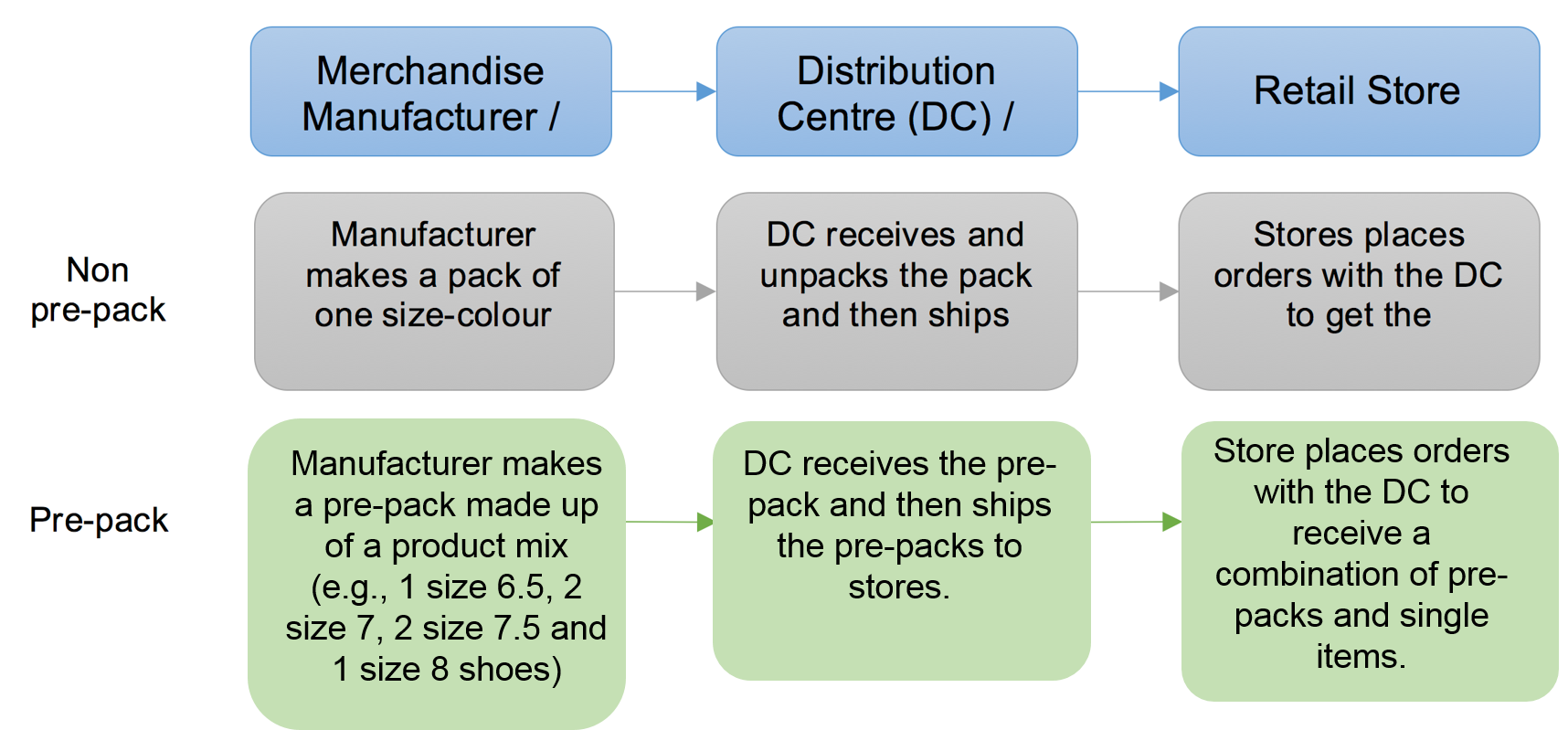
Figure 6: Non pre-packs vs. pre-packs
Graph explaining the relationships between Merchandise Manufacturer / Vendor, Disctibution Centre (DC) / Warehouse and Retail Store.
For the Non pre-pack, the manufacturer makes a pack of one size-colour combination and ships this to the DC (e.g., 40 blue, size 7 shoes). The DC receives and unpacks the pack and then ships single items to stores. The store places orders with the DC to get the inventory they need.
For the pre-pack, the manufacturer makes a pre-pack made up of a product mix (e.g., 1 size 6.5, 2 size 7, 2 size 7.5 and 1 size 8 shoes). The DC receives the pre-pack and then ships the pre-packs to stores. The store places order with the DC to receive a combination of pre-packs and single items.
Short-Term Solvency Ratios
Short-Term Solvency Ratios measure a retailer's ability to meet recurring financial obligations (e.g. bills). A retailer must have sufficient cash flow to prevent defaulting on financial obligations. Liquidity measures short-term solvency and is connected to net working capital, which is current assets minus current liabilities. Current liabilities are debts that must be paid within one year of the date of the balance sheet.
The most common used measures of liquidity are the current ratio and quick ratio.
Current Ratio = Total current assets ÷ Total current liabilities
Quick Ratio = Quick assets ÷ Total current liabilities
If a retailer is in financial trouble, current liabilities may grow faster than current assets and the current ratio may drop. A higher ratio usually means greater liquidity, but a ratio much higher than other retailers may indicate too much inventory or trouble collecting accounts receivables.
Quick assets are current assets that can be quickly converted into cash. Inventory is the least liquid of current assets. It is calculated as (Total Current Assets – Inventory). Compared to the industry average, a high quick ratio helps identify a retailer with too much inventory.
Example
Total current assets of the retailer is $643 million. Total current liabilities is $383 million. Inventory sits at $219 million. What is the current ratio and quick ratio of the retailer?
Solution
Current Ratio = Total current assets ÷ Total current liabilities Current Ratio = $643 ÷ $383 Current Ratio = 1.68 Quick Ratio = Quick Assets ÷ Total Current Liabilities Quick Ratio = (Total Current Assets − Inventory) ÷ Total Current Liabilities Quick Ratio = ($643 − $219) ÷ $383 Quick Ratio = 1.11
SKU Rationalization
Over the past decade, retailers have added large numbers of SKUs to their product assortments as they try to create a unique experience and increase sales for their products. For example, the average number of SKUs in a supermarket is now over 50,000.
Retailers are challenged with SKUs consuming a finite amount of space and capacity, that is increasing costs in the supply chain – including the front store, backroom, and warehouse.
In fact, some research indicates that more options can actually decrease consumer sales. It has been suggested that retailers are over SKU'd by as much as 30%. For average retailers, up to 35-40% of total inventory is considered non-performing: slow moving SKUs, with a contribution to sales of less than 5%. Retailers are now trying to reduce the number of items sold and displayed in store, while still satisfying consumer wants. One of the ways to reduce unnecessary inventory is to conduct SKU rationalization.
SKU Rationalization is a systematic process for analyzing, evaluating and determining what SKUs should be part of a store assortment in order to better align with a retailer's strategies, objectives and goals. Typically, most retailers conduct an annual process to evaluate their SKU assortment.
The benefits of SKU Rationalization are:
- Identify profitable SKUs and rank them from highest to lowest.
- Improve product availability with fewer out of stocks.
- A systematic process to evaluate the benefit (revenue and profitability) of stocking individual SKUs.
- Reduce supply chain costs (inventory and shipping).
- Make room for new products.
Key Components of the SKU Rationalization Process are:
- Define short and long-term company strategies, objectives and goals.
- Analyze SKU performance on the basis of metrics such as sales, gross margin, space productivity, stock turnover, stock-to-sales ratio, and shelf life.
- Review SKU assortment implications such as market share, competitive position, category goals.
- Finalize SKU deletions and implement new assortment.
SKU Selection
While quantitative data is important in making assortment decisions for the SKU rationalization process, there are a number of other qualitative decisions that should be considered to deliver the optimal assortment for the shelf.
The key is to come to an improved assortment of SKUs using a combination of quantitative data, analysis, experience, intuition and strategic thought.
The final SKU selection process should consider a number of other factors such as:
- The strategic role of each item, brand, and section in the category:
- Do the SKUs create traffic in the stores?
- Do the SKUs provide the variety that customers are looking for?
- Do the SKUs fill a product niche that provides a competitive advantage?
- Do the SKUs make a price statement?
- Seasonal and local variations:
- How different are the seasons and climate where stores are located?
- How different are customers between store locations? What are the demographics of local customers?
- Contributions from Vendors:
- Has the vendor provided marketing dollars to promote the SKUs?
- Market Basket implications with loyal shoppers:
- Is the SKU popular with repeat buyers? Would it anger them if the SKU was no longer available?
- Market Basket implications among "early adopter" and "influencer" shoppers:
- Does the SKU bring in customers that can influence market decisions?
- Substitutability:
- How easily can the SKU be substituted by a different SKU?
SKU Selection is best conducted by a combination of the vendor and the retailer, working together to consider the competing interests and factors. The goal is to maximize sales and margin by creating the best shopping experience for customers.
Stock Turnover
Decisions that buyers make with respect to sales and inventory planning must generate a profit for the retailer. The stock turnover rate measures how well sales are balanced to inventory levels. How fast items are sold, replenished, and sold again determines the stock turnover. The stock turnover rate is the number of times the average stock is sold during a period of time and is calculated as:
Stock Turnover Rate = Sales ÷ Average Stock
The average stock for a time period is the value of inventory at the start of the period, plus the value of inventory at a certain period (i.e. end of month), plus the value of inventory at the end of the period divided by the total number of inventory periods.
Higher stock turnover rates are usually better for a retailer because fast turnover of stock reduces the amount of markdowns required to sell off old items.
Example
Calculate stock turnover based on the following information:
Total sales = $20,000
| Month | Month # | Retail |
|---|---|---|
| Jan 31 | 1 | $5,000 |
| Feb 28 | 2 | $8,000 |
| Mar 31 | 3 | $10,000 |
| Apr 30 | 4 | $8,000 |
| May 31 | 5 | $7,000 |
| June 30 | 6 | $9,000 |
| Total Inventory | $47,000 |
Solution
1. First calculate the average monthly inventory:
Average Stock = Total Inventory ÷ Number of Months
Average Stock = $47,000 ÷ 6
Average Stock = $7,833
2. Next calculate the stock turnover rate:
Stock Turnover Rate = Sales ÷ Average Stock
Stock Turnover Rate = $20,000 ÷ $7,833
Stock Turnover Rate = 2.6
Stock-to-Sales Ratio
After forecasting sales, the allocation analyst needs to plan the inventory levels needed to meet the sales that have been predicted. As an analyst, the goal is to ensure that inventory at each store is sufficient for sales in each location without overstocking the store.
Allocation analysts conduct significant research to understand their inventory needs. They often study sales patterns for stores in certain locations to decide how much inventory is necessary.
The most often used method of inventory planning is the stock-to-sales ratio. The stock-to-sales ratio maintains inventory at a certain ratio to sales. Stock-to-sales ratios are calculated by dividing the value of stock on hand by actual sales in dollars. For example, if a department has inventory valued at $50,000 at the beginning of May and sales of $25,000, the stock-to-sales ratio would be 2.
Example
The inventory in the Coffee & Tea department is valued at $90,000. Sales in September is $30,000. What is the stock-to-sales ratio?
Solution
Stock-to-sales ratio = Value of stock ÷ Actual sales
Stock-to-sales ratio = $90,000 ÷ $30,000
Stock-to-sales ratio = 3
Store Ranking Target Groups
If you have not worked through Module 4: Developing a New Store Plan already, please refer to the business situation in that module for further context on this topic.
The next part in determining the appropriate stores for selection is to generate the metrics that will allow a retailer to rank stores against the target groups identified in the trade area segmentation.
The trade area segmentation analyzes all 68 distant trade area (market) segments against the 18 potential store locations. However, the data needs to be aggregated and analyzed for only the 12 segments that comprise the fast fashion retail segments – the Suburban and Urban Cores.
The metrics provided in the trade area segmentation can be used to create the store ranking target groups. The ranking is comprised of three parts:
- Segmentation data by store location for the base region (GTA),
- Suburban Core segments and
- Urban Core segments.
The Suburban and Urban segments can be compared to the base region to determine the magnitude of potential demand for each store for both core segments.
The three metrics that need to be ranked are the %, the % Pen, and Index, for both the Suburban Core and Urban Core segments. Note that a store can only be in one segment (Suburban or Urban).
The following table provides definitions of the column metrics and calculations.
| Column metric | Definition | Calculation |
|---|---|---|
| Base Count (B) | The total population within 3 km of store location in the GTA | Sum of Count by store |
| Base % (C) | The percentage of the base count to the total population | Base Count ÷ Total GTA Base Count × 100 |
| % Suburban Core in GTA (D) | The percentage of Suburban Core households in all of the GTA | Sum of Count of Suburban Core ÷ Total GTA Base Count × 100 |
| % Urban Core in GTA (E) | The percentage of Urban Core households in all of the GTA | Sum of Count of Urban Core ÷ Total GTA Base Count × 100 |
| Count (F) | Number of Suburban Core Households in store's trade area | Sum of Count of Suburban for Store Location |
| % (G) | % of Count of all Suburban Core Segments | Sum of Count of Suburban for Store Location ÷ Sum of Count of all Suburban Stores |
| % Ranking (H) | Ranking of the each store's % of Count | Rank of % |
| % Pen (I) | % of Suburban Core Households in store's trade area (Penetration) | Base Count ÷ Count × 100 |
| % Pen Ranking (J) | Ranking of each store's % Pen | Rank of % Pen |
| Index (K) | Comparison between the Suburban Core Base % and the Suburban Core Segments % for the specific trade area. A value under 100 is considered to be under indexed. A value above 100 is considered to be over indexed. | % Pen ÷ % Suburban Core in GTA |
| Index Ranking (L) | Ranking of each store's Index | Rank of Index |
Trade Area Demographics
Trade Areas Defined
- Retailers need to understand their customers and the markets within which they operate their store locations.
- A trade area is a geographical market definition concept that explicitly captures the area in which a location (e.g., a retail store) derives "most" of its patronage (i.e., customers).
- No commonly accepted definition of a trade area. Typically contiguous areas that contain the majority of customers or potential customers that use or may interact with a supply point.
Types of Trade Areas
- Deterministic (all-or-nothing) versus Probabilistic (likelihood of patronage) Trade Areas
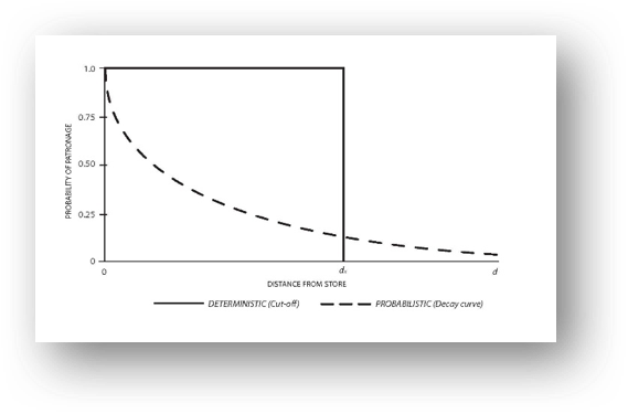
Figure 7: Distance Decay Chart (Source: Toronto Metropolitan University)
This chart shows a decreasing curve from left to right as the probability of patronage drops when the distance from the store increases.
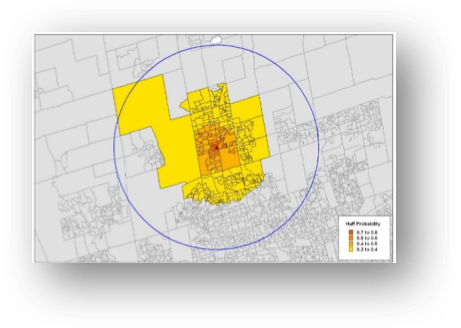
Figure 8: Distance Decay Map (Source: Toronto Metropolitan University)
This arial view of a store on a map uses colour gradients to show that probability of patronage drops (i.e., the colour gets lighter) when the distance from the store increases.
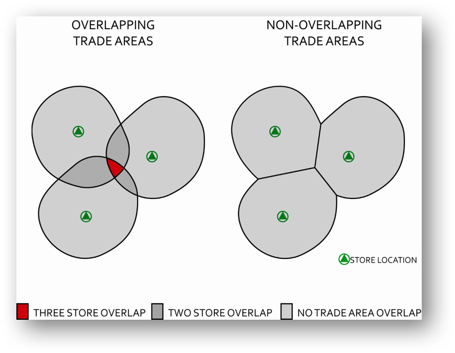
Figure 9: Overlapping and non-overlapping trade areas (Source: Toronto Metropolitan University)
Primary, Secondary and Tertiary Trade Area
While a trade area captures the area from which a store derives most of its customers, a retailer may choose to differentiate between different types of trade area based on the notion of distance decay (i.e., patronage decreases with distance from the store):
- Primary – the core customer area (e.g., a 2.5 km concentric circle around the store)
- Secondary (e.g., between 2.5-5 km from the store)
- Tertiary (e.g., 5-10 km)
Four Basic Deterministic Commonly-Used Trade Area Methods
- User-Drawn (vary depending on the analyst)
- The "Classic" Circular Trade Area (i.e., concentric buffers)
- Percentage of Customers
- Travel cost (e.g. drive time)
The "Classic" Circular Trade Area (i.e., Concentric Buffers)
- A simple circle drawn around a store at a set radius (e.g., 3 km), with customers either "inside" or "outside" of the circle.
- Everyone within X km is as likely to frequent the store regardless of distance. Customer beyond X are assumed never to shop at the store.
- "As the crow flies"(straight line) distance is the most appropriate.
- No physical barriers impede the consumer.
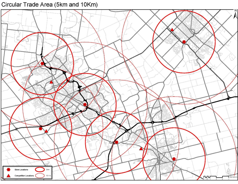
Figure 10: Map of the "classic" circular trade Area (Source: Toronto Metropolitan University)
Percentage of Customers
- Requires information on a store-by-store basis of the location of customers (e.g., postcode, street address).
- Customer locations for a given store are mapped around the store.
- The distance of each customer to the store is calculated and then sorted from closest to furthest distance to the store.
- The trade area is defined as the X % of closest customers to the store. For example the closest 60% are the primary trade area, 60-80% secondary, and 80-90% the tertiary market.
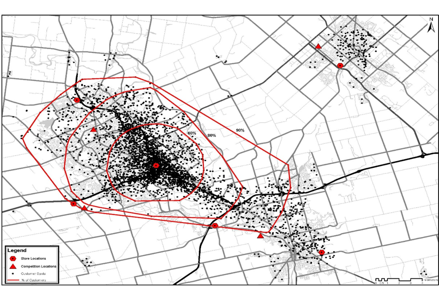
Figure 11: Map of the percentage of customers (Source: Toronto Metropolitan University)
Drive Time
- A road network is needed that has information about how long it takes to travel along each segment of road.
- Drive times are calculated by selecting the roads segments that can be reached within a given time frame, e.g., 5 or 10 minutes.
- The trade area is defined as the shape that bounds the selected road segments.
- Drive times can be adjusted for traffic congestion conditions, for example, peak vs. off-peak drive times.

Figure 12: Road network and drive time (Source: Toronto Metropolitan University)
Comparison of Basic Deterministic Trade Area Approaches
| Trade Area Technique | User Drawn | Circular | Percentage of Customers | Travel Cost |
|---|---|---|---|---|
| Expertise | Experience-based, relies solely on subjective judgment. Trade areas can vary drastically from analyst to analyst | Experience and rules-of-thumb typically needed to determine radius of circle/s, can also use proportion of customers, or weight by attractiveness | Limited requirements, some basic market research, geocoding and mapping skills | Limited requirements, understanding of underlying transport network, choice of impedance value/ cost metrics |
| Time | Fast (for single trade area), but, extremely slow for a large network of stores | Extremely fast, available as standard function in GIS, and retail software packages | Relatively fast, need access to geocoding software and customer survey data. Extremely slow if customer data needs to be collected | Fast, dependent on complexity of transport network, slower when using multiple transport layers (public and private transport modes) |
| Data Requirements | Basic contextual map(street, physical barriers and boundary data); can leverage customer spotting data to inform size and shape of trade area | Customer data or store attractiveness data sometimes used to determine radius. Technique generally used when customer and other data are not available | Representative customer spotting data, postal/street address data for geocoding purposes | Road network file with impedance values for arcs/nodes. Ideally, need access to data with various impedance value scenarios to reflect different traffic conditions (peak, off-peak, weekend) |
| Applications | Widespread use, often used as a final 'safety-check' when other methods have been adopted. Experienced analysts can produce extremely high quality trade areas, capture trade area anomalies on a store-by-store basis. | Widespread use due to ease of operation, speed and lack of strict data requirements, popular amongst retail property developers. Difficult to apply in situations with many competitors or extensive barriers to travel. | Used extensively within demographic profiling and general retail. Need to ensure that the customer data are representative or results will reflect data collection bias. | Commonly used in demographic profiling applications. |
| Cost | Low (for single site), High (for multiple sites and when spotting data used) | Extremely Low | Medium | Medium High |
Trade Area Summary
- Trade areas are an approximation for the area around the store from which most of its customers are drawn.
- The 'trade area' is a concept, not a physical entity.
- Trade area concepts are based on a number of assumptions regarding the nature of store patronage / consumer behavior. All trade areas have a subjective component.
- Trade area definition techniques are ways of operationalizing trade area concepts.
- Numerous trade definition techniques exist – ranging from user-drawn polygons to modeled store patronage probability models.
- The most widely used approaches include, user-drawn, circular or ring, percentage of customers trade areas, and drive time travel.
Trade Area Demographics
- The trade area maps the geographic size and shape of the area from which the majority of customers are drawn.
- Trade areas can be populated with demographic data to develop an understanding of the consumers that reside within the area.
- Demographic data, typically derived from national government surveys, provide information on many different aspects of the resident population, e.g.:
- population size, no. of households, income levels, age of the maintainer, household type and size, marital status, presence and age of children, level of education, type of occupation, immigrant and visible minority status, languages spoken, housing type and age, mode of travel for commuting, etc.
- Absolute Demographics refer to counts or totals that capture size and scale of the population (very sensitive to trade area definition).
- e.g., Total Population 0-4 years old, Aggregate Household Income, Total Households
- Relative Demographics refer to percentages and ratios that capture the character (or tendency) of the population (less sensitive to trade area definition).
- e.g., Percentage of Population 0-4 years old, Average Household Income, Average Number of Persons Per Household
How to Read Trade Area Demographics
- The trade area is used typically to help understand the existing or potential level of performance of a given store.
- To assess a store network a retailer needs both absolute and relative demographic variables.
- For example, an electronics retailer may need both a given number of households (absolute) with an appropriate percentage of 25-44 year olds and above average income (relative) in order to operate a successful store.
Often retailers compare (index) their stores (the target) to either the overall market or the profile of successful stores (the base).
Trade Area Segmentation
If you have not worked through Module 4: Developing a New Store Plan already, please refer to the business situation in that module for further context on this topic.
Trade Area Segmentation is a market segmentation systems that classifies neighbourhoods based on their socioeconomic and geodemographic compositions. This system classifies consumers using many of the variables that can distinguish consumer behavior, from household characteristics such as social group and lifestage, to other traits like income, family status, age of children, education and even housing choice.
Trade Area Segmentation classifies Canadian neighborhoods into 68 distinct trade area (market) segments. Segments with similar characteristics can be grouped together. Trade Area Segmentation combines the "who" of segment characteristics with the "where" of neighbourhood geodemographic to create a model of segments of actual neighbourhoods with distinct behavioral market segments. The analysis identifies potential retailers that match the household profile of the trade area (also referred to as base region).
For fast fashion, there are two core segments – Suburban and Urban. The Suburban Core is made up of a group of 7 segments, while the Urban Core is made up of a group of 5 segments. See Figure 13. Within each core, the segments comprise neighbourhoods with similar buying habits and geodemographic.
The trade area segmentation analysis provides data for a 3 km radius around each of the 18 potential store locations (A to R). All segment data is compared to the base region, which is Toronto (GTA).
For each store location, the segmentation provides four characteristics:
- Count – The population of the segment in a 3 km radius around the store.
- % - The percentage of population of the segment compared to the total of all segments.
- % Pen – The penetration of the population of the segment compared to the base count (total population of segment in base region).
- Index – Comparison between the segment core base % and location segment base % for the specific trade area.
Why Should Retailers Use Trade Area Segmentation?
Retailers need to understand customers so that they can supply them with the right products and reach them with the right form of communication. They also need to know where their customer are so that they can target them with the right location and type of store.
This requires a segmentation system that can profile diverse trade areas. The analysis can determine the requirements that best match the buying habits and geodemographics within a store location's trade area.
Retailers who use trade area segmentation generate trade area maps that display the concentration of customers by location. Ultimately, the goal is to determine the magnitude of potential demand for a retailer's goods within a trade area.

Figure 13: Fast Fashion Target Groups identified by Trade Area Segmentation (Source: Toronto Metropolitan University)
This figure shows the fast fashion target groups branching out into two segments: urban core and suburban core. Each segment is further divided into smaller segments that correspond with environics categories including those with "kids and careers" or "heritage hubs" among others in the suburban core and "urban digerati", "grads & pads" and "newcomers rising" plus others in the urban core.
Visual Merchandising
Visual Merchandising is the process of attracting customers with visual cues.
This is essential to a retailer's ability to generate sales. The way that stores are arranged, the location of displays, the lighting, are all meticulously planned with planograms to generate more sales per square foot.
Store display decisions are based on a wide number of choices as follows:
Merchandise Display Format
- Shelves
- Hanging
- Pegs
- Folded
- Stacked
- Dumped
Merchandise Display Type
- Image – basic/fashion
- Colours
Physical Merchandise Layout
- Store fixture type
- Store location
- Category signage
Planograms enable the retailer to control inventory and maximize shelf space utilization. It helps:
- Improve the visual appearance of the store.
- Improve brand awareness.
- Control inventory to avoid out of stocks.
- Utilize shelf space more efficiently to maximize selling potential.
- Improve financial performance of assortments.
- Manage product replenishment.
- Develop better marketing through targeted displays.
- Increase product sales and margin.